neuromodels.models.HodgkinHuxley¶

class neuromodels.models.HodgkinHuxley(V_rest=- 65.0, Cm=1.0, gbar_K=36.0, gbar_Na=120.0, gbar_L=0.3, E_K=- 77.0, E_Na=50.0, E_L=- 54.4, degC=6.3)[source]¶

Class for representing the original Hodgkin-Huxley model.

The Hodgkin–Huxley model describes how action potentials in neurons are initiated and propagated. From a biophysical point of view, action potentials are the result of currents that pass through ion channels in the cell membrane. In an extensive series of experiments on the giant axon of the squid, Hodgkin and Huxley succeeded to measure these currents and to describe their dynamics in terms of differential equations.

This class implements the original Hodgkin-Huxley model for the sodium, potassium and leakage channels found in the squid giant axon membrane. Membrane voltage is in absolute mV and has been reversed in polarity from the original HH convention and shifted to reflect a resting potential of -65 mV.

All model parameters can be accessed (get or set) as class attributes. Solutions are available as class attributes after calling the class method solve().

Parameters

V_restfloat: Resting potential of neuron in units \(mV\), default=-65.0.
Cmfloat: Membrane capacitance in units \(\mu F/cm^2\), default=1.0.
gbar_Kfloat: Potassium conductance in units \(mS/cm^2\), default=36.0.
gbar_Nafloat: Sodium conductance in units \(mS/cm^2\), default=120.0.
gbar_Lfloat: Leak conductance in units \(mS/cm^2\), default=0.3.
E_Kfloat: Potassium reversal potential in units \(mV\), default=-77.0.
E_Nafloat: Sodium reversal potential in units \(mV\), default=50.0.
E_Lfloat: Leak reversal potential in units \(mV\), default=-54.4.
degCfloat: Temperature when recording (should be to set a squid-appropriate temperature) in units \(^{\circ}C\), default=6.3.

Notes

Default parameter values as given by Hodgkin and Huxley [1].

References

1: A. L. Hodgkin, A. F. Huxley, “A quantitative description of membrane current and its application to conduction and excitation in nerve”, J. Physiol. 117, pp. 500-544, 1952.

Examples

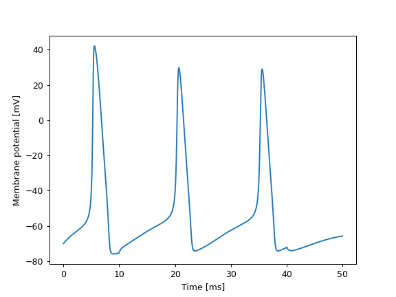
import matplotlib.pyplot as plt
import neuromodels as nm

# Initialize the Hodgkin-Huxley system; model parameters can either
# be set in the constructor or accessed as class attributes:
hh = nm.HodgkinHuxley(V_rest=-70)
hh.gbar_K = 36

# The simulation parameters needed are the simulation time T, the time
# step dt, and the input stimulus, the latter either as a constant,
# callable with call signature `(t)` or ndarray with `shape=(int(T/dt)+1,)`:
T = 50.
dt = 0.025

def stimulus(t):
    return 10 if 10 <= t <= 40 else 0

# The system is solved by calling the class method `solve` and the
# solutions can be accessed as class attributes:
hh.solve(stimulus, T, dt)
t = hh.t
V = hh.V

plt.plot(t, V)
plt.xlabel('Time [ms]')
plt.ylabel('Membrane potential [mV]')
plt.show()

../_images/neuromodels-models-HodgkinHuxley-1.png

Attributes

V_rest	(`float`) Model parameter: Resting potential.
Cm	(`float`) Model parameter: Membrane capacitance.
gbar_K	(`float`) Model parameter: Potassium conductance.
gbar_Na	(`float`) Model parameter: Sodium conductance.
gbar_L	(`float`) Model parameter: Leak conductance.
E_K	(`float`) Model parameter: Potassium reversal potential.
E_Na	(`float`) Model parameter: Sodium reversal potential.
E_L	(`float`) Model parameter: Leak reversal potential.
degC	(`float`) Model parameter: Temperature when recording in degrees Celsius.
t	(ndarray) Solution: Array of time points `t`.
V	(ndarray) Solution: Array of voltage values `V` at `t`.
n	(ndarray) Solution: Array of state variable values `n` at `t`.
m	(ndarray) Solution: Array of state variable values `m` at `t`.
h	(ndarray) Solution: Array of state variable values `h` at `t`.

Methods

`I_K`(V, n)	Potassium current.
`I_L`(V)	Leak current.
`I_Na`(V, m, h)	Sodium current.
`__call__`(t, y)	RHS of the Hodgkin-Huxley ODEs.
`alpha_h`(V)	Sodium channel inactivation forward reaction rate.
`alpha_m`(V)	Sodium channel activation forward reaction rate.
`alpha_n`(V)	Potassium channel activation forward reaction rate.
`beta_h`(V)	Sodium channel inactivation backward reaction rate.
`beta_m`(V)	Sodium channel activation backward reaction rate.
`beta_n`(V)	Potassium channel activation backward reaction rate.
`h_inf`(V)	Sodium channel inactivation steady state.
`m_inf`(V)	Sodium channel activation steady state.
`n_inf`(V)	Potassium channel activation steady state.
`solve`(stimulus, T, dt[, y0, method])	Solve the Hodgkin-Huxley equations.
`tau_h`(V)	Sodium channel inactivation time constant.
`tau_m`(V)	Sodium channel activation time constant.
`tau_n`(V)	Potassium channel activation time constant.

I_K(V, n)[source]¶

Potassium current.

Parameters

Vfloat or ndarray: Membrane potential.
nfloat or ndarray: Potassium channel state variable.

Returns

I_Kfloat or ndarray: Potassium current.

I_Na(V, m, h)[source]¶

Sodium current.

Parameters

Vfloat or ndarray: Membrane potential.
mfloat or ndarray: Sodium channel activation state variable.
hfloat or ndarray: Sodium channel inactivation state variable.

Returns

I_Nafloat or ndarray: Sodium current.

I_L(V)[source]¶

Leak current.

Parameters

Vfloat or ndarray: Membrane potential.

Returns

I_Lfloat or ndarray: Leak current.

alpha_n(V)[source]¶

Potassium channel activation forward reaction rate.

Uses the vtrap() function to trap for zero in denominator of rate equation.

Parameters

Vfloat or ndarray: Membrane potential.

Returns

ratefloat or ndarray: Reaction rate.

beta_n(V)[source]¶

Potassium channel activation backward reaction rate.

Parameters

Vfloat or ndarray: Membrane potential.

Returns

ratefloat or ndarray: Reaction rate.

alpha_m(V)[source]¶

Sodium channel activation forward reaction rate.

Uses the vtrap() function to trap for zero in denominator of rate equation.

Parameters

Vfloat or ndarray: Membrane potential.

Returns

ratefloat or ndarray: Reaction rate.

beta_m(V)[source]¶

Sodium channel activation backward reaction rate.

Parameters

Vfloat or ndarray: Membrane potential.

Returns

ratefloat or ndarray: Reaction rate.

alpha_h(V)[source]¶

Sodium channel inactivation forward reaction rate.

Parameters

Vfloat or ndarray: Membrane potential.

Returns

ratefloat or ndarray: Reaction rate.

beta_h(V)[source]¶

Sodium channel inactivation backward reaction rate.

Parameters

Vfloat or ndarray: Membrane potential.

Returns

ratefloat or ndarray: Reaction rate.

n_inf(V)[source]¶

Potassium channel activation steady state.

Parameters

Vfloat or ndarray: Membrane potential.

Returns

steady_statefloat or ndarray: Steady state.

tau_n(V)[source]¶

Potassium channel activation time constant.

Parameters

Vfloat or ndarray: Membrane potential.

Returns

time_constantfloat or ndarray: Time constant.

m_inf(V)[source]¶

Sodium channel activation steady state.

Parameters

Vfloat or ndarray: Membrane potential.

Returns

steady_statefloat or ndarray: Steady state.

tau_m(V)[source]¶

Sodium channel activation time constant.

Parameters

Vfloat or ndarray: Membrane potential.

Returns

time_constantfloat or ndarray: Time constant.

h_inf(V)[source]¶

Sodium channel inactivation steady state.

Parameters

Vfloat or ndarray: Membrane potential.

Returns

steady_statefloat or ndarray: Steady state.

tau_h(V)[source]¶

Sodium channel inactivation time constant.

Parameters

Vfloat or ndarray: Membrane potential.

Returns

time_constantfloat or ndarray: Time constant.

solve(stimulus, T, dt, y0=None, method='RK45', **kwargs)[source]¶

Solve the Hodgkin-Huxley equations.

The equations are solved on the interval (0, T] and the solutions evaluted at a given interval. The solutions are not returned, but stored as class attributes.

If multiple calls to solve are made, they are treated independently, with the newest one overwriting any old solution data.

The solver only accepts stimulus as either a scalar (int or float), callable or ndarray. If callable, the call signature must be one and only one positional argument, e.g. (t). Kewword arguments are allowed in passed callables. When passed as ndarray, stimulus must have shape (int(T/dt)+1).

Parameters

stimulus{int, float}, callable or ndarray, shape=(int(T/dt)+1,)

Input stimulus in units \(\mu A/cm^2\). If callable, the call signature must be (t).

Tfloat

End time in milliseconds (\(ms\)).

dtfloat

Time step where solutions are evaluated.

y0array_like, shape=(4,)

Initial state of state variables V, n, m, h. If None, the default Hodgkin-Huxley model’s initial conditions will be used; \(y_0 = (V_0, n_0, m_0, h_0) = (V_{rest}, n_\infty(V_0), m_\infty(V_0), h_\infty(V_0))\).

methodstr

Integration method to use. Description from the scipy.integrate.solve_ivp documentation:

‘RK45’ (default): Explicit Runge-Kutta method of order 5(4) [1]. The error is controlled assuming accuracy of the fourth-order method, but steps are taken using the fifth-order accurate formula (local extrapolation is done). A quartic interpolation polynomial is used for the dense output [2]. Can be applied in the complex domain.

‘RK23’: Explicit Runge-Kutta method of order 3(2) [3]. The error is controlled assuming accuracy of the second-order method, but steps are taken using the third-order accurate formula (local extrapolation is done). A cubic Hermite polynomial is used for the dense output. Can be applied in the complex domain.

‘DOP853’: Explicit Runge-Kutta method of order 8 [13]_. Python implementation of the “DOP853” algorithm originally written in Fortran [14]_. A 7-th order interpolation polynomial accurate to 7-th order is used for the dense output. Can be applied in the complex domain.

‘Radau’: Implicit Runge-Kutta method of the Radau IIA family of order 5 [4]. The error is controlled with a third-order accurate embedded formula. A cubic polynomial which satisfies the collocation conditions is used for the dense output.

‘BDF’: Implicit multi-step variable-order (1 to 5) method based on a backward differentiation formula for the derivative approximation [5]. The implementation follows the one described in [6]. A quasi-constant step scheme is used and accuracy is enhanced using the NDF modification. Can be applied in the complex domain.

‘LSODA’: Adams/BDF method with automatic stiffness detection and switching [7], [8]. This is a wrapper of the Fortran solver from ODEPACK.

**kwargs

Arbitrary keyword arguments are passed along to scipy.integrate.solve_ivp.

Notes

The ODEs are solved numerically using the function scipy.integrate.solve_ivp.

If stimulus is passed as an array, it and the time array, defined by T and dt, will be used to create an interpolation function via scipy.interpolate.interp1d.

solve_ivp is an ODE solver with adaptive step size. If the keyword argument first_step is not specified, the solver will empirically select an initial step size with the function select_initial_step (found here https://github.com/scipy/scipy/blob/master/scipy/integrate/_ivp/common.py#L64).

This function calculates two proposals and returns the smallest. It first calculates an intermediate proposal, h0, that is based on the initial condition (y0) and the ODE’s RHS evaluated for the initial condition (f0). For the standard Hodgkin-Huxley model, however, this estimated step size will be very large due to unfortunate circumstances (because norm(y0) > 0 while norm(f0) ~= 0). Since h0 only is an intermediate calculation, it is not used or returned by the solver. However, it is used to calculate the next proposal, h1, by calling the RHS. Normally, this procedure poses no problem, but can fail if an object with a limited interval is present in the RHS, such as an interp1d object.

In the case of the standard Hodgkin-Huxley model, one might be tempted to pass the stimulus as an array to the solver. In order for solve_ivp to be able to evaluate the stimulus, it must be passed as a callable or constant. Thus, if an array is passed to the solver, an interpolation function must be created, in this implementation done with interp1d, for solve_ivp to be able to evaluate it. For the reasons explained above, the program will hence terminate unless the first_step keyword is specified and is set to a sufficiently small value. In this implementation, first_step=dt is already set in solve_ivp.

The solve_ivp keyword max_step should be considered to be specified for stimuli over short time spans, in order to ensure that the solver does not step over them.

Note that first_step still needs to specified even if max_step is. select_initial_step will be called regardless if first_step is not specified, and the calls for calculating h1 will be done before checking whether h0 is larger than than the max allowed step size or not. Thus will only specifying max_step still result in program termination if stimulus is passed as an array. (Will not be a problem in this implementation since first_step is already specified.)

References

1: J. R. Dormand, P. J. Prince, “A family of embedded Runge-Kutta formulae”, Journal of Computational and Applied Mathematics, Vol. 6, No. 1, pp. 19-26, 1980.
2: L. W. Shampine, “Some Practical Runge-Kutta Formulas”, Mathematics of Computation,, Vol. 46, No. 173, pp. 135-150, 1986.
3: P. Bogacki, L.F. Shampine, “A 3(2) Pair of Runge-Kutta Formulas”, Appl. Math. Lett. Vol. 2, No. 4. pp. 321-325, 1989.
4: E. Hairer, G. Wanner, “Solving Ordinary Differential Equations II: Stiff and Differential-Algebraic Problems”, Sec. IV.8.
5: Backward Differentiation Formula on Wikipedia.
6: L. F. Shampine, M. W. Reichelt, “THE MATLAB ODE SUITE”, SIAM J. SCI. COMPUTE., Vol. 18, No. 1, pp. 1-22, January 1997.
7: A. C. Hindmarsh, “ODEPACK, A Systematized Collection of ODE Solvers,” IMACS Transactions on Scientific Computation, Vol 1., pp. 55-64, 1983.
8: L. Petzold, “Automatic selection of methods for solving stiff and nonstiff systems of ordinary differential equations”, SIAM Journal on Scientific and Statistical Computing, Vol. 4, No. 1, pp. 136-148, 1983.

API Reference neuromodels.utils.compute_q10_correction