neuromodels.models.HodgkinHuxley¶

class neuromodels.models.HodgkinHuxley(V_rest=- 65.0, Cm=1.0, gbar_K=36.0, gbar_Na=120.0, gbar_L=0.3, E_K=- 77.0, E_Na=50.0, E_L=- 54.4)[source]¶

Class for representing the Hodgkin-Huxley model.

The Hodgkin–Huxley model describes how action potentials in neurons are initiated and propagated. From a biophysical point of view, action potentials are the result of currents that pass through ion channels in the cell membrane. In an extensive series of experiments on the giant axon of the squid, Hodgkin and Huxley succeeded to measure these currents and to describe their dynamics in terms of differential equations.

All model parameters can be accessed (get or set) as class attributes. Solutions are available as class attributes after calling the class method solve().

Parameters

V_restfloat: Resting potential of neuron in units \(mV\), default=-65.0.
Cmfloat: Membrane capacitance in units \(\mu F/cm^2\), default=1.0.
gbar_Kfloat: Potassium conductance in units \(mS/cm^2\), default=36.0.
gbar_Nafloat: Sodium conductance in units \(mS/cm^2\), default=120.0.
gbar_Lfloat: Leak conductance in units \(mS/cm^2\), default=0.3.
E_Kfloat: Potassium reversal potential in units \(mV\), default=-77.0.
E_Nafloat: Sodium reversal potential in units \(mV\), default=50.0.
E_Lfloat: Leak reversal potential in units \(mV\), default=-54.4.

Notes

Default parameter values as given by Hodgkin and Huxley (1952).

References

Hodgkin, A. L., Huxley, A.F. (1952). “A quantitative description of membrane current and its application to conduction and excitation in nerve”. J. Physiol. 117, 500-544.

Examples

>>> import matplotlib.pyplot as plt
>>> from pylfi.models import HodgkinHuxley

Initialize the Hodgkin-Huxley system; model parameters can either be set in the constructor or accessed as class attributes:

>>> hh = HodgkinHuxley(V_rest=-70)
>>> hh.gbar_K = 36

The simulation parameters needed are the simulation time T, the time step dt, and the input stimulus, the latter either as a constant, callable or ndarray with shape=(int(T/dt)+1,):

>>> T = 50.
>>> dt = 0.025
>>> def stimulus(t):
...    return 10 if 10 <= t <= 40 else 0

The system is solved by calling the class method solve and the solutions can be accessed as class attributes:

>>> hh.solve(stimulus, T, dt)
>>> t = hh.t
>>> V = hh.V

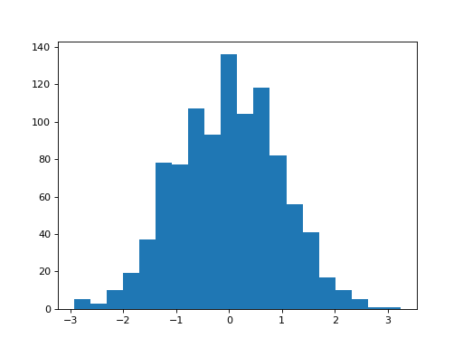
>>> plt.plot(t, V)
>>> plt.xlabel('Time [ms]')
>>> plt.ylabel('Membrane potential [mV]')
>>> plt.show()

(Source code, png, hires.png, pdf)

../_images/neuromodels-models-HodgkinHuxley-1.png

another

(Source code)

Attributes

V_restfloat: Model parameter: Resting potential.
Cmfloat: Model parameter: Membrane capacitance.
gbar_Kfloat: Model parameter: Potassium conductance.
gbar_Nafloat: Model parameter: Sodium conductance.
gbar_Lfloat: Model parameter: Leak conductance.
E_Kfloat: Model parameter: Potassium reversal potential.
E_Nafloat: Model parameter: Sodium reversal potential.
E_Lfloat: Model parameter: Leak reversal potential.
tndarray: Solution: Array of time points t.
Vndarray: Solution: Array of voltage values V at t.
nndarray: Solution: Array of state variable values n at t.
mndarray: Solution: Array of state variable values m at t.
hndarray: Solution: Array of state variable values h at t.

Methods

`__call__`(t, y)	RHS of the Hodgkin-Huxley ODEs.
`solve`(stimulus, T, dt[, y0])	Solve the Hodgkin-Huxley equations.

solve(stimulus, T, dt, y0=None, **kwargs)[source]¶

Solve the Hodgkin-Huxley equations.

The equations are solved on the interval (0, T] and the solutions evaluted at a given interval. The solutions are not returned, but stored as class attributes.

If multiple calls to solve are made, they are treated independently, with the newest one overwriting any old solution data.

Parameters

stimulus{int, float}, callable or ndarray, shape=(int(T/dt)+1,): Input stimulus in units \(\mu A/cm^2\). If callable, the call signature must be (t).
Tfloat: End time in milliseconds (\(ms\)).
dtfloat: Time step where solutions are evaluated.
y0array_like, shape=(4,): Initial state of state variables V, n, m, h. If None, the default Hodgkin-Huxley model’s initial conditions will be used; \(y_0 = (V_0, n_0, m_0, h_0) = (V_{rest}, n_\infty(V_0), m_\infty(V_0), h_\infty(V_0))\).
**kwargs: Arbitrary keyword arguments are passed along to scipy.integrate.solve_ivp.

Notes

The ODEs are solved numerically using the function scipy.integrate.solve_ivp.

If stimulus is passed as an array, it and the time array, defined by T and dt, will be used to create an interpolation function via scipy.interpolate.interp1d.

solve_ivp is an ODE solver with adaptive step size. If the keyword argument first_step is not specified, the solver will empirically select an initial step size with the function select_initial_step (found here https://github.com/scipy/scipy/blob/master/scipy/integrate/_ivp/common.py#L64).

This function calculates two proposals and returns the smallest. It first calculates an intermediate proposal, h0, that is based on the initial condition (y0) and the ODE’s RHS evaluated for the initial condition (f0). For the standard Hodgkin-Huxley model, however, this estimated step size will be very large due to unfortunate circumstances (because norm(y0) > 0 while norm(f0) ~= 0). Since h0 only is an intermediate calculation, it is not used or returned by the solver. However, it is used to calculate the next proposal, h1, by calling the RHS. Normally, this procedure poses no problem, but can fail if an object with a limited interval is present in the RHS, such as an interp1d object.

In the case of the standard Hodgkin-Huxley model, one might be tempted to pass the stimulus as an array to the solver. In order for solve_ivp to be able to evaluate the stimulus, it must be passed as a callable or constant. Thus, if an array is passed to the solver, an interpolation function must be created, in this implementation done with interp1d, for solve_ivp to be able to evaluate it. For the reasons explained above, the program will hence terminate unless the first_step keyword is specified and is set to a sufficiently small value. In this implementation, first_step=dt is already set in solve_ivp.

The solve_ivp keyword max_step should be considered to be specified for stimuli over short time spans, in order to ensure that the solver does not step over them.

Note that first_step still needs to specified even if max_step is. select_initial_step will be called regardless if first_step is not specified, and the calls for calculating h1 will be done before checking whether h0 is larger than than the max allowed step size or not. Thus will only specifying max_step still result in program termination if stimulus is passed as an array. (Will not be a problem in this implementation since first_step is already specified.)

API Reference